Cloud-native data centre network security. Ouch, that’s a mouthful isn’t it?

The lengthy phrase precisely captures the complexity of what we’re dealing with here: to secure the network of a cloud-native infrastructure (e.g. Kubernetes), running on top of an on-premise data centre. This topic may sound foreign as it is usually broken into smaller pieces such as the security of a data centre network, VPC, Kubernetes network, or container network.

Cloud native data centre networking heavily relies on network virtualisation, which dramatically differs from those traditional models (like the famous access-aggregation-core architecture, more on this later). Just like how virtual machines run on a shared host. Network virtualisation allows people to stack multiple layers of virtualised networks to form a greater scale of network that had never been achieved before (figure 0). As we know with great complexity comes great vulnerability, the complication of the cloud native network naturally creates lots of security implications. But the real danger is, many organisations are still using the traditional approach to secure their cloud native infrastructure without noticing that their firewall/IDS/IPS/network policy may have failed silently.

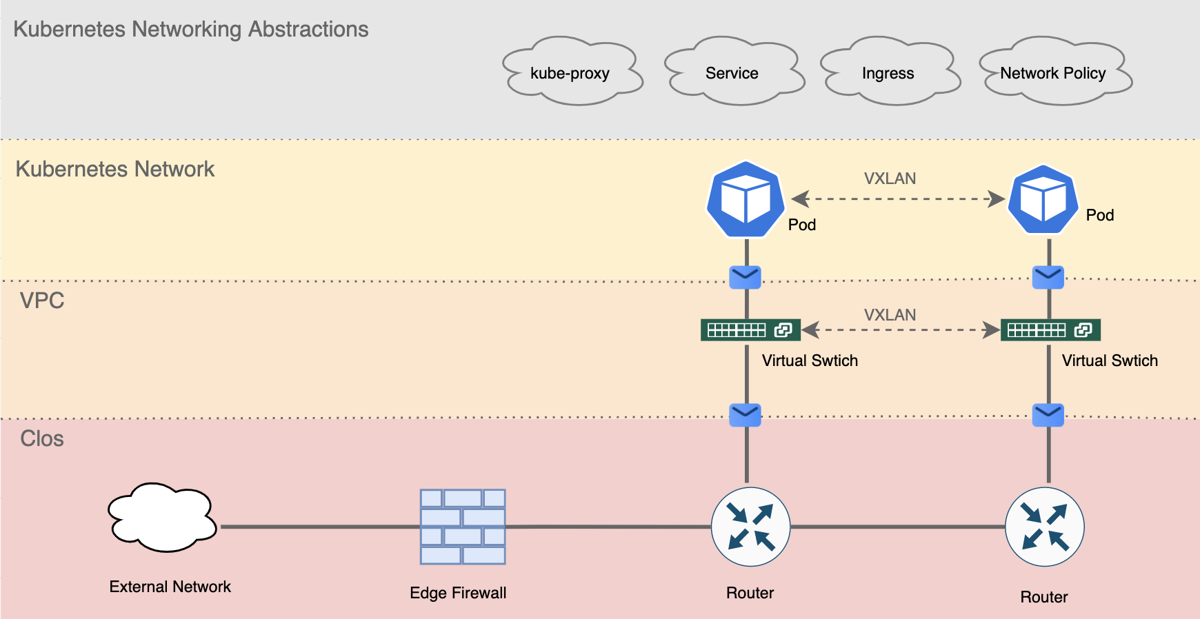
Figure 0. Layers of network abstractions in a cloud native data centre

This post aims to introduce the chaotic world of cloud native data centre networking and network virtualisation. We will focus on a particular type of network virtualisation, namely the overlay network,* which constitutes an essential part of a cloud native data centre in the modern days. Kubernetes will be used as an example throughout the piece to set a practical context for discussions. We will discuss Kubernetes networking abstractions and their security implications in the later parts of the series.

*Inline Network vs Overlay Network There’re two types of network virtualisation, namely the inline network and the overlay network. Inline network implies the idea that every hop in the network is aware of the underlying virtual network, and uses this knowledge to make routing decisions. Examples of an inline network are VLAN and VRF. On the contrary, the overlay network means only edge nodes of a network are aware of the virtual network and makes routing decisions while the other intermediate nodes blindly forward packets. VXLAN is an example of such an overlay network.

Traditional Data Centre Networking #

Let’s recap on the traditional data centre architecture. In a pre-cloud setting, the software runs in either physical servers or VMs. Because there is no microservice, workloads are usually self-contained within one or a few machines. Most of the network traffic therefore happens between the Internet and the servers. As you can see from the the figure below, the traffic traverse through the network infrastructure vertically. In networking jargon, this is called north-south traffic.

The architecture, named access-aggregation-core or access-agg, comprises several layers.

• Servers at the bottom, are connected to the access switch, which in turn connected to another aggregation switch. Notice both connections are on Layer 2 (bridging) instead of Layer 3 (routing). In other words, servers connected under the same aggregation switch can send packets to each other based on MAC addresses*.
• Aggregation switch then connects to a core router where Layer 3 routing happens (based on IP addresses)**
• When traffic needs to the exit core router and enters the Internet, it has to pass through the edge firewall (“the firewall”) and reach the edge router. The edge router then forwards the traffic to the uplink ISP
• Notice every layer comprised of two or more identical devices for high availability(HA) purpose
• VLAN is the most common technique used to further divide the network into several isolated L2 networks.

*To keep things simple, here we ignore VLANs and assume there’s only one Layer 2 broadcast domain.

**Assume L2/L3 boundary is at the aggregation link. A popular variant of access-agg architecture moves L2/L3 boundary to the core router layer, but it’s out of the scope of our discussion.

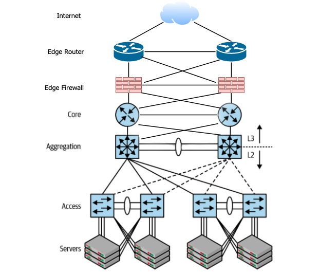
Figure 1. Access-aggregation-core network architecture. Notice that this is a logical view of the network. The actual cabling and device placement may vary. Picture modified from source[1]

Traditional firewalls make perfect sense in this design. Being the only chokepoint in the north-south traffic force all packets to go through the scrutiny of the firewall. More importantly, a physical server or VM only runs one service. The firewall can use the internal IP of the machine to reliably identify the underlying services and to apply appropriate rules.

Entering Cloud Native Data Center #

The rise and fall of access-aggregation-core #

Access-agg had its moment. Don’t get me wrong. You’ll still see it around in small to medium-sized networks but not any more in any big data centres of the tech giants. Given the rise of microservice, the prominent traffic pattern in data centres is changing from north-south to east-west, meaning the server-to-server traffic within the data centre is much more than the traffic goes in and out of the data centre. The huge east-west traffic puts significant pressure on the aggregation switches and core switches, making them soon become the bottleneck of the entire network.

Other than the capacity issue, access-agg also has many other drawbacks.

• VLAN limitation: A 12-bit long VLAN ID only allows a maximum of 4096 VLANs in a network. Imagine your are a public cloud provider and each of your users needs 1 VLAN for his/her isolated network. You’ll run out of VLAN IDs shortly after serving 4000+ customers.
• L2 Flooding: bridges use a “flood-and-learn” model to learn new MAC addresses, and they do it periodically due to timeouts. Flooding thousands of machines in a big L2 network can significantly degrade the network performance.
• Limitation of STP: In access-agg architecture, every VLAN needs to run a separate spanning tree protocol (STP) instance to create its L2 routing table. However, STP won’t work with more than two aggregation switches. This limits the bandwidth of the aggregation layer.
• Failure Domain: If a switch/router/firewall goes down in our illustrated network above, the network bandwidth is immediately reduced to half. The blast radius is simply too large for any cloud infrastructure.
• Complexity: The actual complexity of access-agg is way beyond our scope of discussion. A multitude of additional protocols are required to keep the network running, such as STP, FHRP, VLAN, and VTP. Network engineers need to plan very carefully for every change in the network so as not to disturb any of the moving parts.

Clos Network #

If not access-agg, what’s our next bet? Entering Clos network. Clos topology isn’t an entirely new concept. It was first invented in the 1950s to switch telephone calls! 70 years later, Clos has found itself a new home in the modern data centre.

The idea of Clos topology is rather simple: build two layers of switches namely the spine and the leaf (Figure 2). Make every leaf connect to every spine switch to form a fully-meshed network. The leaf switch is usually placed on top of a rack(ToR), which connects to the rest of the servers in the same rack (Figure 3).

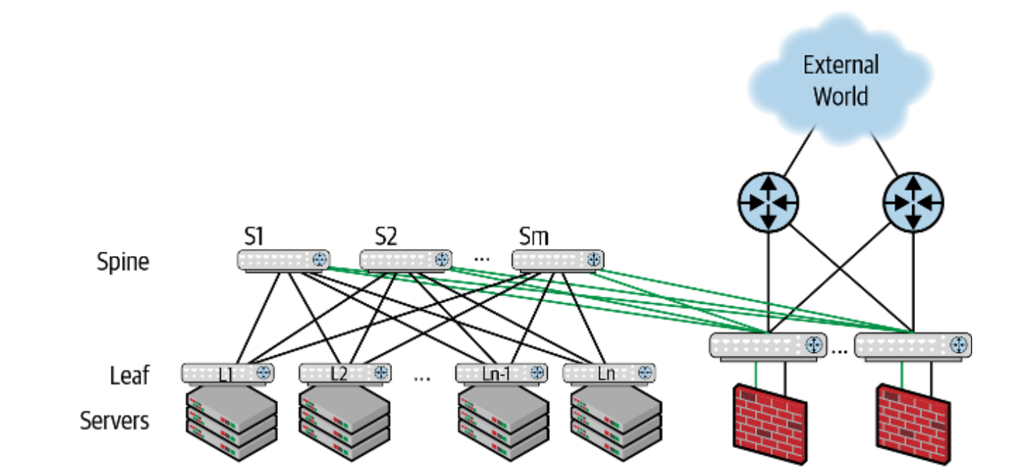
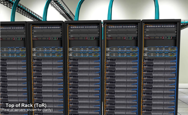
Figure 3. A typical Clos network rack. Each rack has a leaf node with two Top of Rack(ToR) switches in the middle (with blue cables).https://www.kareemccie.com/2017/09/what-is-difference-between-top-of-rack.html

One of the most fundamental differences between access-agg and Clos is that Clos embraces routing as the fundamental mode of connections, meaning bridging only happens at the leaf node within a rack. Any other traffic between leaf-leaf or leaf-spine will default to routing. Inter-leaf routing usually uses BGP, but that’s outside of our scope of discussion.

Clos topology has several advantage when running cloud native workloads.

• Simplified Routing: Clos is essentially a fully meshed network as every spine connects to every leaf. Hence, a leaf can pick any of the spines to reach to another leaf. This is the so-called the Equal-Cost Multipath (ECMP) routing
• Increased bandwidth: east-west traffic now have multiple equal-weight paths to travel through which implies a much higher bandwidth
• Better redundancy: a single switch failure only reduces a fraction of the overall bandwidth but won’t affect the overall connectivity
• Use of homogeneous switches: Clos topology encourages people to build large networks by using small fixed-form-factor switches. This simplifies inventory management and facilitates network automation.

In a real-world scenario, you should more often see a three-tier Clos design. By adding another layer of switches on top (known as super-spine), Clos topology can scale further to support more servers.* The figure below should give you a rough idea of what Facebook, Microsoft, and Amazon’s data centre looks like.

*The formula used to calculate the maximally supported servers in a two-tier Clos network is n^2/2 where n is the number of switch ports. Assume all leaf and spine nodes use the same switch. Hence if we use 64-port switches, the total number of connected servers is 64^2/2 = 2048. This is a physical limitation because a fully meshed network needs a lot of ports to build inter-connectivity (e.g. a leaf needs x ports to connect to x spines).

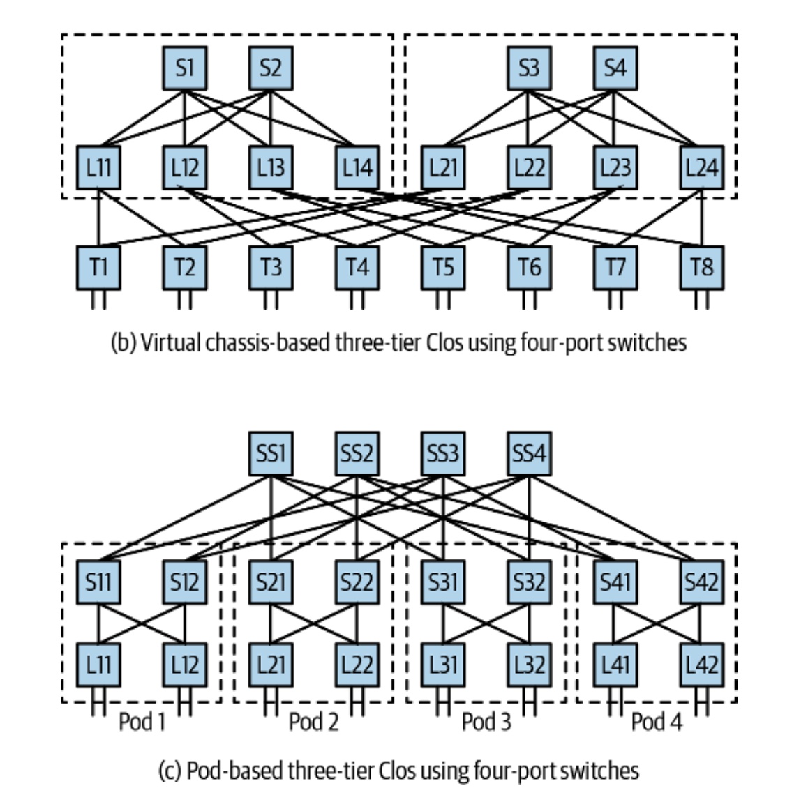
Figure 4. Two typical three-tier Clos network topologies. (b) is used by Facebook. (c) is used by Microsoft and Amazon. Source[1]

Understanding Network Virtualisation #

The Clos topology so far looks elegant. However, an astute reader may have noticed: we can’t use VLAN anymore! Imagine if we have a customer who rents two racks of servers and needs to put them in the same Layer 2 network. Intuitively, you may want to put all servers in a VLAN, like those good old days. However, you can’t possibly create a VLAN that spans two leaves in Clos. Remember bridging in Clos is restricted to only a leaf switch and its servers within the same rack? A Layer 2 VLAN encapsulated datagram simply can’t travel through the Layer 3 link between the two leaf switches.

Luckily, we have VXLAN coming to rescue. But this changes everything.

Introducing VXLAN #

VXLAN is a rather new protocol that only came in 2014 as RFC7348 but quickly became the backbone of almost every single cloud vendor. In short, VXLAN is an L2 tunnel protocol that operates on top of an L3 network. In other words, VXLAN is like a VLAN-over-IP alternative. It allows any number of servers to form a virtual L2 network by encapsulates L2 datagrams in UDP packets, and send it over an IP network like normal UDP traffic (Figure 5).

Just like VLAN has a VLAN ID, VXLAN uses a VXLAN Network Identifier(VNI) to differentiate tunnels. The end of a tunnel that charges encapsulating and decapsulating packets is called Virtual Tunnel Endpoint(VTEP). VTEP could be either a virtual interface or a physical switch, as long as it understands VXLAN.

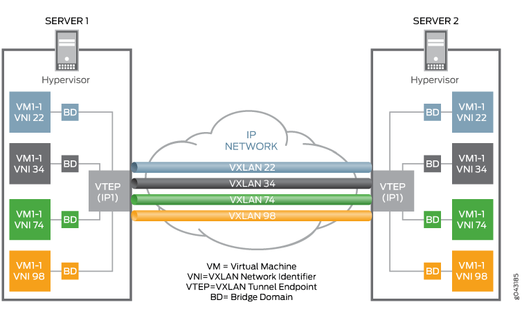
Figure 5. Overview of VXLAN. Source[3]

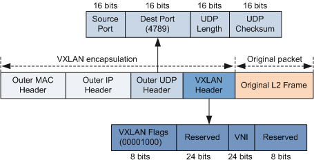
Figure 6. VXLAN header format. Source[5]

In the public cloud, VXLAN has become the de facto standard for VPC networks. If you create a VPC on AWS*/GCP/Azure/AliCloud**, you’re essentially creating an overlay VXLAN on top of the cloud vendor’s infrastructure. Thanks to the 24-bit VNI, a Clos network could now run 2^24=16777216 VXLANs in parallel as long as the computational power allows.

*The well-known AWS VPC isn’t exactly VXLAN, but it’s built on a very similar implementation.[6] Notice at the time when AWS released VPC in 2009 there was no VXLAN yet. VXLAN only came in 2014.

**AliCloud made themselves clear that their VPC uses VXLAN. https://www.alibabacloud.com/zh/product/vpc

VXLAN in Kubernetes #

If you’re building a cloud native infrastructure, there’s a high chance that you’ll set up a Kubernetes cluster on top of the VPC. Kubernetes as a container orchestration platform acts as an abstraction layer for all underlying computational resources, whether or not it’s CPU, memory, or network.

The networking model in Kubernetes is built entirely around the concept of the overlay network. By abstracting away the details in the underlying hardware, the overlay network becomes the one and only logical representation of your actual network topology. The benefit? You can define whatever network topology in code and deploy it on any Kubernetes clusters on AWS, GCP, or even your own data centres. The infrastructure-as-code approach makes network upgrade, troubleshooting, and migration a lot easier and more flexible.

The magical power of Kubernetes networking again is built on top of VXLAN*. Kubernetes manage its own networking by creating another VXLAN network among all nodes (Figure 7). The actual traffic between pods and services are therefore proxied through VXLAN tunnels. You may be surprised to find out that all nodes in a Kubernetes cluster are fully connected in this VXLAN layer. The lack of control of such flat topology, being remarkably similar to the Clos network, is essentially a deliberate design that purposefully relinquishes the network control to the upper layer of network abstractions (such as Kubernetes’ NetworkPolicy).

*For most of the network plugins such as flannel, weave-net, and Cillium.

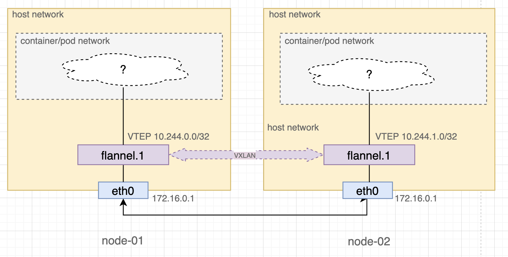
Figure 7. VXLAN tunnel between two Kubernetes nodes with flannel

Kubernetes provides a variety of overlay network implementations through network plugins. We can have a peek at the internals through one of the popular choices named flannel. As you saw above, flannel runs a flannel.x VTEP interface on every Kubernetes node. Through flannel.x, flannel establishes a one-to-one VXLAN tunnel with every other node to form a virtualised L2 network. Whenever a new node joins the cluster, flannel adds two records to all existing nodes, namely:

• ARP record of the remote node’s VTEP interface. The record comprises a pair of the remote VTEP’s IP and MAC address.
• VXLAN fdb record of the remote node which maps the remote VTEP’s MAC address to the remote node’s IP

If a pod wishes to talk to another pod on a remote node, the combination of the two records translate the destination pod’s internal IP (in the remote VTEP’s IP range) → remote VTEP’s MAC → remote node’s IP. flannel.x interface then can encapsulate the packet and ask eth0 to forward it to the right node.

Pod/Container Network #

Let’s dig deeper to see how pods talk to each other through the overlay network.

In Kubernetes, a pod may contain one or more containers. Also, a pod represents a shared network namespace. Because of the isolation of network namespaces, containers in a pod has to rely on a veth(https://man7.org/linux/man-pages/man4/veth.4.html), a virtual Ethernet device, to communicate with the host network. For example, in the figure below, eth0 in container A pairs up with vethxxxxxx to create a bridged tunnel between namespaces. All veth interfaces on the same host then connect to a virtual bridge named cni0, which in turn connects to the VTEP flannel.x so as to talk to the external world.

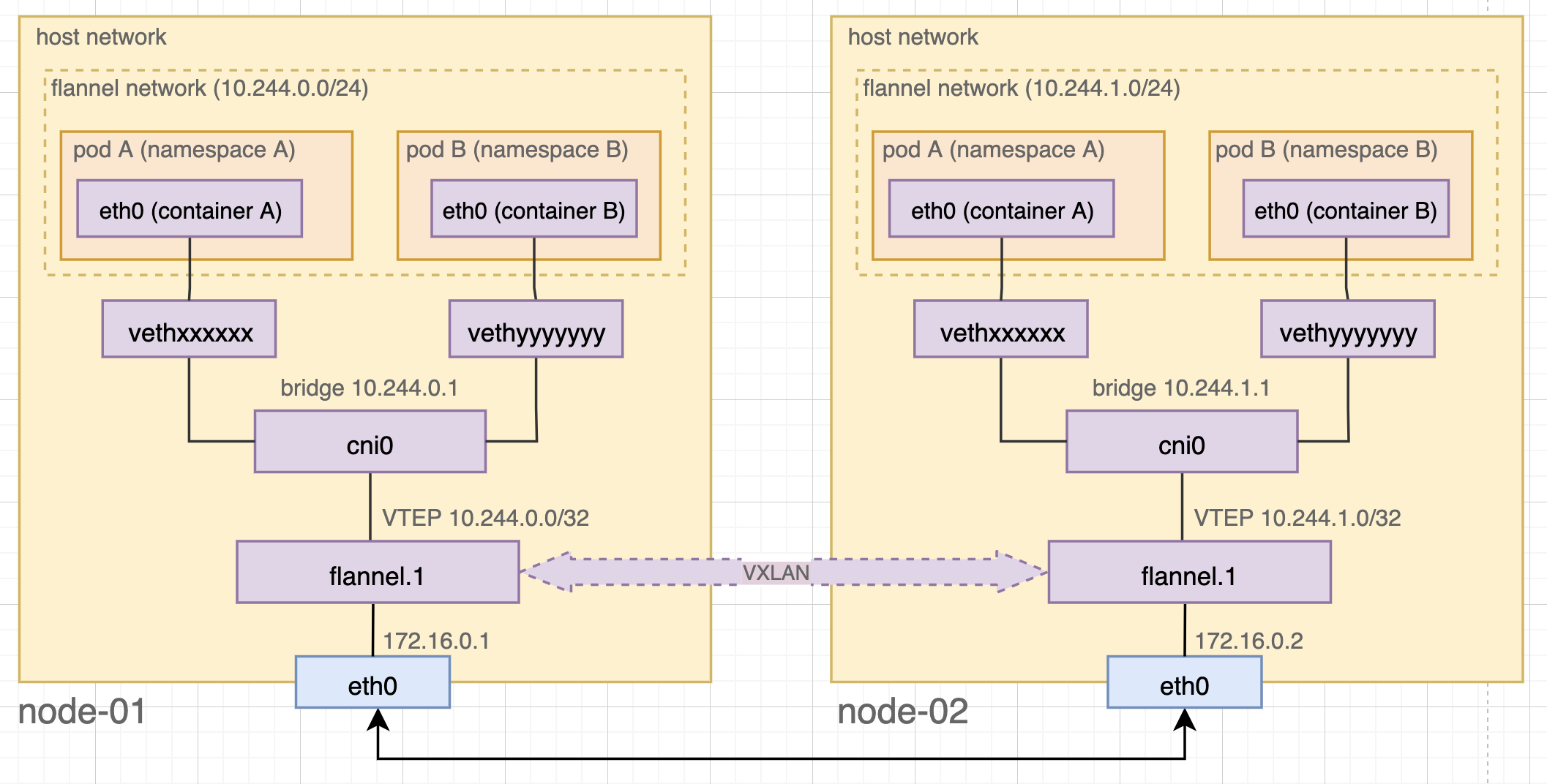
Figure 8. Kubernetes networking with flannel

The Bigger Picture #

This had been a long journey! So far we have travelled from the Clos network in the data centre, through VPCs in the middle, and eventually landed in the mysterious overlay network in Kubernetes.

Imagine you have two microservices running in two separate Kubernetes pods. Two pods are scheduled to two different Kubernetes nodes on two different VMs in the VPC network. And the two VMs are situated in two different physical machines respectively. For one service to talk to the other, it needs to know:

• The IP address of the destination pod in the Kubernetes internal network
• The pod runs on a Kubernetes node, which is on a virtual machine in the VPC network. Hence we need to know the destination pod’s VM’s address
• The VM’s VPC network is an isolated Layer 2 domain, running as a VXLAN on top of the physical Clos network. Because the Clos network is connected through routing, we need to know the destination host machine’s IP address

In fact, any data packets exchanged between these services have three nested layers of TCP/IP headers*! Networking in a cloud native data centre is a complicated topic because of these many layers. Any security decision, like where to put a firewall, now have to think thrice. There’s a high chance that a security mechanism in the lower layer won’t regulate virtualised traffic running on top of it.

*More precisely, it’s one plain TCP/IP packet wrapped under two more layers of VXLAN header.

Just like how shift-left revamps DevOps, we need to start thinking about moving network security defence to the upper layer of the virtualised infrastructure. But before diving into the details, we will have to understand how Kubernetes makes use of this virtualised infrastructure to build its own networking kingdom. And that’s one more layer of abstractions.

References #

1. Cloud Native Data Center Networking, Dinesh G. Dutt, O’Reilly 2020
2. What is the difference between Top of Rack and End of Row, Mahmmad, Kareemoddin, 2017, Source: https://www.kareemccie.com/2017/09/what-is-difference-between-top-of-rack.html
3. VXLAN Data Center Interconnect Using EVPN Overview, Juniper Network, 2021, Source: https://www.juniper.net/documentation/us/en/software/junos/evpn-vxlan/topics/concept/vxlan-evpn-integration-overview.html
4. RFC7348 - Virtual eXtensible Local Area Network (VXLAN): A Frameworkfor Overlaying Virtualized Layer 2 Networks over Layer 3 Networks, 2014, Source: https://datatracker.ietf.org/doc/html/rfc7348
5. Huawei DCN Design Guide, Huawei, 2018, Source: https://support.huawei.com/enterprise/en/doc/EDOC1100023542?section=j016&topicName=vxlan
6. A Day in the Life of a Billion Packets (CPN401) | AWS re:Invent 2013, AWS, 2013, Source: https://www.youtube.com/watch?v=Zd5hsL-JNY4&t=942s
7. Flannel Network Demystify, Huang Yingting, 2018, Source: https://msazure.club/flannel-networking-demystify/
8. Understanding Weave Net, Weaveworks, Source: https://www.weave.works/docs/net/latest/concepts/how-it-works/
9. Comparing Kubernetes CNI Providers: Flannel, Calico, Canal, and Weave, Rancher, 2019, Source: https://rancher.com/blog/2019/2019-03-21-comparing-kubernetes-cni-providers-flannel-calico-canal-and-weave/
10. Cluster Networking, Kubernetes documentation, Source: https://kubernetes.io/docs/concepts/cluster-administration/networking/